A Bit Of History

This blog post is based on one of my favorite papers of all time: “A New Interpretation of Information Rate” (Kelly, 1956). The paper, written by John L. Kelly, derives a formula for gambling optimally which is now known as the “Kelly Criterion”. Mathematician turned hedge fund manager, Ed Thorpe, is famously known for using this formula at his hedge fund. Thorpe’s fund outperformed the S&P500 by a factor of ~3 over a span of 20 years (Fortunesformula.com, n.d.).

If after reading this post you want to learn more about the history of this formula, I highly recommend (Poundstone, 2010). In it, you can read about how Thorpe and Shannon created the first wearable computer to beat the casinos at roulette, how Thorpe beat the casinos at blackjack, and how he later moved on to opening up a hedge fund.

The Problem Setup

We will study the following problem:

There is biased coin and you know its probability of landing heads is .6. Someone offers you the chance to bet as much money as you want on the outcome of a toss of the biased coin. The bet is 1-to-1 odds (if you bet 10 dollars and lose, you lose those 10 and if you win you end up with 20 dolars in your pocket). You can play this game for 100 rounds. How much money should you bet in each round?

Now, stop reading and think about how much you would bet. Seriously, take your time to think about it. Write it down in a piece of paper.

I’ve asked this question to many people and very few (~15%) get something that is roughly right. Most people end up leaving a lot of money on the table and unfortunately many people, some with PhDs in probability related fields, go bust.

Let’s first answer a simpler question: Should you even bet at all? If you bet $x$ dollars on heads your expected payoff is $p_{win} * x + p_{lose} (-x) = .6x - .4x = .2x$ dollars, which is positive, so yes, you should definetely bet (on heads!). Let $W_0$ be your initial wealth and $f \in [0, 1]$ the fraction of your wealth that you are going to bet. Your expected wealth after the first round of gambling is:

$\underbrace{W_0(1-f)}_{\text{the amount of wealth you don't bet}} + \underbrace{(.6) * 2 W_0 f}_{\text{probability of winning $\times$ prize if you win}} + \underbrace{(.4) * 0}_{\text{probability of losing $\times$ prize if you lose}}$

This simplifies to $W_0 + .2 W_0 f$, which is a simple linear function which is maximized at $f^* = 1$. So, to maximize your expected wealth you should bet your entire wealth in the first round…

Well, this is idiotic for obvious reasons, we don’t want to lose all our hard-earned savings in a single round of a stupid game! But somehow “the math” is telling us to do so… Let this be a lesson to not always follow what the math says, or what some “expert” using fancy math says. Always think and analyze by yourself, make sure your results align with your intuition. And if you are going to use math to justify high-stake decisions you better understand the math really well!

So, why are we getting an obviously wrong answer if our math is “correct”? My take is that this is just an artifact of the definition of expected value, the definition itself (together with taking the maximum) does not capture the aspect of reality that we want it to capture. –>

Finding the Optimal Fraction to Bet

Before we do the math to figure out how much to actually bet, let’s set up some notation so that we can apply our learnings to similar problems. Let $W_i$ be your wealth in round $i$ (your initial wealth is $W_0$), $u$ be your % gains if you win the bet, $d$ your % loses if you lose the bet, $p$ the probability of winning the bet, and $q = 1-p$ be the probability of losing the bet. In our biased coin example we have $p=.6, q=.4, u=1$, and $d=1$.

Let’s compute our wealth $W_1$ in the scenario where the coin lands on heads. We decided to wager $W_0 f$ dollars and since we won the bet we’ve turned that into $W_0 f (1+u)$, at the same time we kept $W_0 (1-f)$ in our pocket, so $W_1 = W_0 f (1+u) + W_0 (1-f) = W_0 (1+f u)$. Similarly, if the coin lands tails $W_1$ would be: $W_0 (1- f d)$. It is not too hard to see that our wealth in the last round will be equal to:

$W_{100} = W_0 (1+fu)^{\text{numberOfHeads}}(1-fd)^{\text{numberOfTails}},$

where $\text{numberOfHeads}$ is the number of times we got heads in the 100 rounds we played, and $\text{numberOfTails}$ is defined similarly. In expectation $\text{numberOfHeads} = 100 p$ and $\text{numberOfTails} = 100 q$. So we want to maximize

$W_0 (1+fu)^{100 p}(1-fd)^{100 q} \tag{1}.$

Taking natural logs on both sides of the equation we have

$\ln(W_0)+ 100 p \ln(1+fu) + 100 q \ln(1-fd).$

This is for sure a concave function on $f$ as long as $d < 1$ i.e. we can’t lose more than we actually bet (I’ll let you double check the second derivative). So we can take the gradient with respect to $f$ and set it equal to 0.

$\frac{100pu}{(1+f^*u)} - \frac{100qd}{1-f^*d} = 0.$

Solving for $f^*$ we get

$f^* = \frac{p}{d} + \frac{q}{u}.$

This is the formula that is known as the Kelly Criterion. In our example, $u=d=1$, $p=.6$, so we get that $f^* = .2$, according to the formula we should be betting $20$ % of your wealth in every round. Moreover, plugging in the optimal solution into equation (1) where 100 is replaced with $T$ rounds we get:

$W_0 (1.2)^{.6T} (.8)^{.4T} = W_0 e^{log(1.2^{.6T})} e^{log(.8^{.4T})} \approx e^{.02T},$

which means we should expect our wealth to grow exponentially fast!

This time we’ve arrived at an answer that actually makes sense. If we get unlucky and get a few tails in a row we won’t go broke, but it is aggressive enough to grow our wealth at an exponential rate.

Below is a plot of how much you should expect your wealth to grow by at the end of 100 rounds when you bet a constant fraction of it in every round. This is equation (1) in the case where $u=d=1$, and $p=.6$. If we bet $20$ % in every round we expect to grow our wealth by a factor of 7.5, not bad at all! But we have to be careful, if we bet more than $38$ % we will start loosing money, and if we are too aggressive and bet more than $50$ % in each round we will lose all our money!

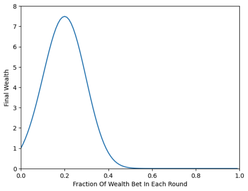
Tread carefully though, as I will show you later in some simulations, growing your money this quickly is not a walk in the park, using this betting strategy comes with big wealth swings.

You should be wondering how is it that the “math” gave us something reasonable this time. Careful inspection of the steps above will show you that this time we are solving $\max_{f \in [0,1]} \mathbb{E}[\ln(W_{100})]$, whereas the first time we were solving $\max_{f \in [0,1]} \mathbb{E}[W_{100}]$. What a big difference using logs makes in finance!

Learnings From Kelly

There are a few simple heuristics we can extract from Kelly’s formula. I think they are useful if you like games of chance, or if you happen to invest (gamble) in the stock market:

1. When you have a bad streak, you reduce how much money (in dollar terms) you are betting. In particular, you don’t double down! If you are one of those who like doubling down when you are losing, or keeps doubling down when a stock keeps going down I beg you to watch this.
2. Never gamble/invest all your money, if you lose it all you won’t have the chance to recover, even when you have an edge!
3. If $u = d$ and $p=q$ i.e. the game is even odds, $f^*$ is equal $0$. Do not bet if you don’t have an edge!

Simulations

Let’s now simulate a few trajectories where we bet $20$% of our wealth in each round. By the way, you can find the code for these plots here. Each trajectory shows our wealth across all 300 rounds of the game:

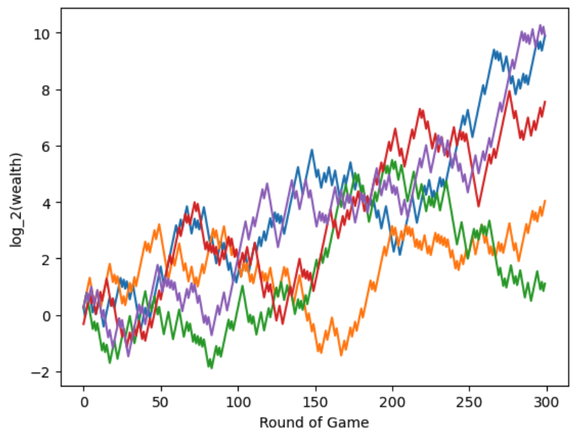
In the $y$-axis I’m using $log_2$, so a value greater than 0 means our wealth is larger than when we started, a value of 1 means we 2x our wealth, a value of 2 means we 4x it and so on, similarly a value of -1 means we lost half of it -2 means we lost $\frac{3}{4}$ of it etc. Focus on the values at 300 rounds, the green line is ~1 so in that trajectory we doubled our money, in the blue and purple trajectories we increased it by a factor of $2^{10} = 1024$, nice.

Notice however, that there is a lot of variance. Focus on the orange line, at round 50 you’ve 8x your wealth, you are ecstatic. Then by step 150 you have lost nearly 60 % of your initial wealth! Imagine starting with 100K, getting all the way up to 800K only to go back to 40K, really wild ride. Even knowing that you were betting optimally, would you have stomached it? Not sure I would have… This is why some people often don’t use full-Kelly and instead use half-Kelly, e.g. they bet $\frac{1}{2}f^*$, this results in lower variance and drawdowns, the cost is a slower rate growth in wealth.

After seeing the plot above I wondered if I’d made a mistake so I plotted a histogram of the final wealth when we play 100 rounds:

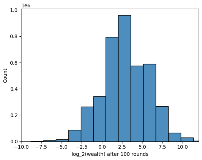
The mean $log_2-$wealth was ~2.9 and $2^2.9 = 7.46$ which matches our expected growth factor. Notice the variance is huge, in ~18% of the trajectories you end up losing money. Additionally, there are some trajectories in which you end up with 1000 times more than what you started with!

It is important to remember that in this life we only live one trajectory, so gamble accordingly.

The Cost of Being Wrong

Before we conclude, let me show you what happens when we are actually wrong about the probability of heads. Imagine that the actual probability of heads is .52, but we (for some reason) think it’s actually .6 so we decide to bet 20% of our wealth in every round, as Kelly says. This is what our wealth would look like in 10 trajectories:

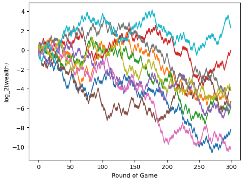
There is only one lucky trajectory where we make money, in most of the other ones we are just setting our money on fire. So, if you are going to use full-Kelly make sure the parameters of the problem are what you think they are!

Disclaimer: The content provided on this blog is for educational purposes only and is not intended to be financial advice. The views and opinions expressed here are solely those of the authors and should not be construed as professional financial advice. Readers are encouraged to consult with a qualified financial advisor before making any financial decisions based on the information provided on this blog.