A Brief Review of Modern Portfolio Theory

A short summary of Modern Portfolio Theory (Markowitz, 1952) is the following. The “risk” of a portfolio is measured by its variance and its “reward” is measured by the expected value of the portfolio itself. Now fix the value of variance, it is possible there are many portfolios with variance equal to the fixed value, MPT tells us that among all these portfolios we should pick the one with the largest expected value (which makes sense).

More formally, if there are $n$ assets with (random) returns $r_i$ where $\mu_i = \mathbb{E}[r_i]$ for $i \in [n]$, the covariance matrix is given by $\Sigma$, and $w_i$ is the fraction of our portfolio we allocate to asset $i \in [n]$, then it is easy to check that the expected return of our portfolio is given by $\mu^\top w$ and its variance is given by $w^\top \Sigma w$, where $\mu$ and $w$ are the vectors of returns and weights. So, for a given portfolio variance, $\sigma^2_{portfolio}$, we need to solve the following optimization problem:

\begin{align} \max_{w} \thinspace & \mu^\top w \cr s. t.\thinspace & w^\top \Sigma w = \sigma^2_{portfolio} \cr & 1^\top w = 1. \tag{1} \end{align}

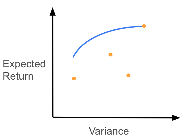
Note we are allowing the portfolio to short certain stocks by not enforcing $w \geq 0$. These portfolios are called “efficient”, and if we plot the maximum expected value portfolio for every possible value of the variance, we get what is called the “efficient frontier” as the following image shows.

As a side note, you may be familiar with the following formulation for finding efficient portfolios:

\begin{align} \max_{w} \thinspace & \mu^\top w - \lambda w^\top \Sigma w, \cr s. t.\thinspace &1^\top w = 1. \tag{2} \end{align}

where $\lambda$ expresses the risk preferences of the portfolio manager. This formulation and the one I presented in (1) are equivalent (I’ll let you prove it yourself).

Our ultimate goal when we are thinking about portfolio construction, is to actually build a portfolio, yet MPT has not provided us one. MPT has given us a set of portfolios that seem to be reasonable (in a later section I will show with an example that not all of them are), and academics will tell you that the right portfolio to pick will depend on each person’s risk preferences. But I have never met anyone who can actually describe their risk preferences… Additionally, in this setting, risk preferences must be specified as a value for the variance of the portfolio, but it is possible to have a large variance due to really large gains, so a large variance is not necessarily a bad thing.

Our goal is to build a portfolio, unfortunately we have not been able to do so. In a previous post, we discussed how to bet optimally on the outcome of a biased coin using the Kelly criterion. Is there a way we can apply those learnings to building portfolios? Before we answer these questions let me convince you that there can be portfolios in the efficient frontier that will ruin you.

Some Efficient Portfolios Lead To Ruin

Consider the “economy” where we have two assets. The first asset doubles your investment with probability .6 and fully loses your investment with probability .4, so $\mu_1 = \mathbb{E}[r_1] = .2$. The second asset guarantees you will not make or lose any money so $\mu_2 = 0$. In this economy the covariance matrix is all zeros except for the top left entry which has the value .96. Plugging these values into (2) to get an efficient portfolio we need to solve

\begin{align} \max_{\lVert w \rVert = 1} .2 w_1 - \lambda .96 w_1^2. \end{align}

Setting the derivative w.r.t. $w_1$ equal to 0 and solving for it we get $w_1=\frac{1}{9.6 \lambda}$. In the previous post we saw that choosing to bet more that 38% of our wealth in the coin will most certainly lead us to ruin in the long run. So, picking any risk preference parameter lambda such that $\frac{1}{9.6 \lambda} > .38$ gives us an efficient portfolio that will lead us to ruin. This is a short cautionary tale to be careful when picking parameters for high-stake decision problems.

Using the Kelly Criterion for Portfolio Construction

Let us assume our initial wealth is 1, let $o_i = 1 +r_i$ for $i \in [n]$, so that $\sum_{i \in [n]}o_i w_i = o^\top w$ is the random variable expressing our wealth.

In this post we showed that when a coin is biased in our favor and the bets are even odds, it is possible to grow our wealth exponentially quickly by maximizing the expected log wealth, and that this is the fastest growth rate. So, why don’t we do the same for portfolio construction? That is, what happens when we use the optimal solution to the following optimization problem

\begin{align} \max_{w} & \mathbb{E}[\ln(o^\top w)] \tag{3}, \end{align}

as the weights for our portfolio? How does this portfolio compare to those prescribed by MPT? Is the Kelly portfolio any good?

I will show shortly, under certain conditions, $w^*$ the solution to (3), which I call the Kelly portfolio, is a good approximation to one of the portfolios in the efficient frontier. Then I will state two important properties that the Kelly portfolio has.

The discussion that follows comes from (Thorp, 1975) and (Breiman, 1961). I highly recomend you read them as I skip details. Also, since I’m rederiving results myself so I can internalize them, the notation may not be consistent with the one in these papers.

The Kelly Portfolio Is (Sometimes) In The Efficient Frontier

We now establish the connection between the Kelly portfolio and MPT. Using the Taylor series expansion: $f(x) = f(y) + \frac{f’(y)(x-y)}{1!} + \frac{f’‘(y)(x-y)^2}{2!} + \frac{f’’‘(y)(x-y)^3}{3!}+…$ of $\ln$ around $(1+\mu)^\top w$. We get

\begin{align} &\ln(o^\top w) \cr &= \ln((1+r)^\top w) \cr &= \ln((1+\mu)^\top w) + \frac{1}{2(1+\mu)^\top w} ((1+r)^\top w - (1+\mu)^\top w) - \cr & \qquad \frac{1}{2((1+\mu)^\top w)^2} ((1+r)^\top w - (1+\mu)^\top w)^2 + \text{h.o. terms}. \end{align}

If we ignore the higher order terms, take expectation, and simplify a bit we have

\begin{align} \mathbb{E}[\ln(o^\top w)] &\approx \ln((1+\mu)^\top w) - \frac{1}{2((1+\mu)^\top w)^2} \mathbb{E}[(r^\top w - \mu^\top w)^2]. \end{align}

So that when we do not allow leverage, i.e. $1^\top w =1$, and $\mu^\top w$ is small, we have $\ln((1+\mu)^\top w) = \ln(1 + \mu^\top w) \approx \mu^\top w$ and $((1+\mu)^\top w)^2 \approx 1$.

Under all the assumptions, we have that:

\begin{align} \mathbb{E}[\ln(o^\top w)] &\approx \mu^\top w - \frac{1}{2} w^\top \Sigma w. \end{align}

We have shown that if the returns are small and moments > 2 are small, then Kelly portfolio, which maximizes $\mathbb{E}[\ln(o^\top w)]$, is equivalent to the Markowitz portfolio (2), with risk parameter $\lambda = \frac{1}{2}$. Conversely, if the returns of the assets you are considering investing in, have potentially very large gains/loses or have nonnegligible higher moments you should think twice before using MPT and $\lambda = .5$. After all, MPT does not even take as input these higher order moments.

Two Important Properties of the Kelly Portfolio

We’ve shown an nice conection between the Kelly portfolio and MPT. But is the Kelly portfolio actually good? Will it make money?

(Breiman, 1961) showed that, when the market is “favorable” (an equivalent condition to (3) being positive), there are two good properties the Kelly portfolio has (informally):

1. Asymptotically, any portfolio strategy that does not approach the value $\max_{w} \mathbb{E}[\ln(o^\top w)]$ will perform infinitely worse than the Kelly portfolio almost surely.
2. Let $x$ be our desired wealth level, and $\mathbb{E}[T_x(w)]$ the expected number of periods required to exceed our desired wealth level, then as $x\rightarrow \infty$, the Kelly portfolio minimizes $\mathbb{E}[T_x(w)]$.

These properties suggest that using the Kelly portfolio is reasonable. The proofs for these claims are quite long, so I won’t include them here.

Practical Aspects of Portfolio Construction

The discussion so far has been detached from reality. In practice we can’t solve either (2) or (3) because we don’t know the distribution of returns. However, something we can do is to estimate the distribution/parameters from historical data and then plug these estimates into (2) and (3). Notice that by doing this we are assuming the distribution of returns is stationary (which is probably not true). Let’s see what happens when we follow this approach in a simulated market. As usual, you can find the code on Github.

The Markowitz Portfolio Under Gaussian Returns

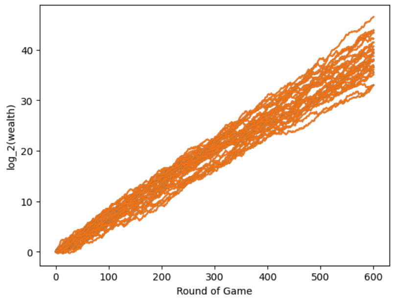
In these simulations we will sample returns from a multivariate Gaussian distribution with $\mu = [0, .05, -.04]$, and

\begin{align} \Sigma = \begin{bmatrix} 0 & 0 & 0 \cr 0 & 0.0101 & 0.009\cr 0 & 0.009 & 0.0164 \end{bmatrix}. \end{align}

The first asset is equivalent to holding cash, the second one is a stock with positive returns, and the last one is a stock with negative returns. The simulation is setup as follows. Using two years of monthly data (24 observations), we estimate the mean returns, and covariance matrix to solve (2) with $\lambda = .5$, to find our portfolio weights. Then we sample from the distribution to get our realized returns, with these we can compute our wealth, and update our mean and covariance estimates. This process repeats for 600 months. The next figure shows in blue 30 wealth trajectories of following this procedure. For each of the aforementioned trajectories we also plot what our wealth would be if we used the true mean and covariance matrix to find the portfolio weights. As you can see, the method of plugging in the estimated parameters works well in this setting.

Unfortunately, the multivariate Gaussian assumption for the returns is not realistic in practice. In the next subsection we explore what happens when the returns are generated from a multivariate Student’s-t distribution.

The Markowitz Portfolio Under Fat Tails

The setup is the same as in the last subsection except that the returns are distributed according to a multivariate Student-t distribution with the same mean and variance as in the previous subsection, and 4 degrees of freedom (still finite variance). The reason for choosing Student’s-t is that it has fatter tails than the Gaussian, so this is a slightly more realistic model.

This is what the trajectories look like:

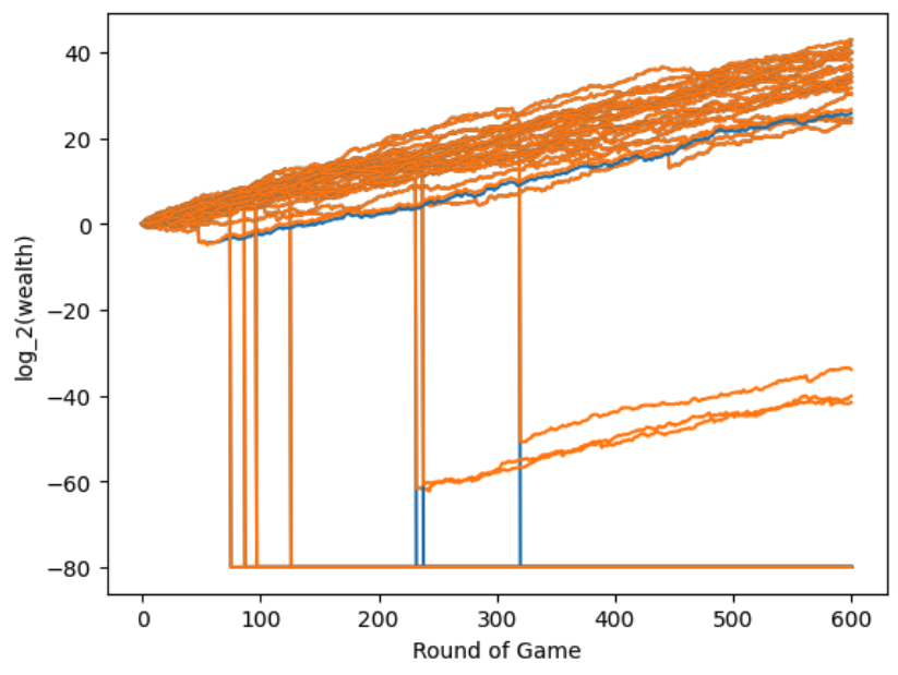
Ouch! See those 7 trajectories where wealth drastically drops? Those drastic losses come from the fat tails of the Student’s t distribution. The large loses don’t show up that often so they don’t really enter into our estimates of mean and variance until it’s too late. But why did this happen? Recall we are using (2) with $\lambda = .5$ to build our portfolio (motivated by the earlier section), but we are no longer in a setting where the higher order (in particular 4-th) moments can be ignored. So, we are obviously over betting. Can this be remedied? This example shows what happens when the Markowitz approximation to the Kelly portfolio fails. What if we solve the Kelly portfolio directly instead of the Markowitz approximation?

The Kelly Portfolio Under Fat Tails

The Kelly portfolio in this example most likely involves betting a very small fraction of your wealth on stock #1 and keeping the remaining fraction of your wealth in cash (just as in the biased coin example from the last post). To determine the actual fraction we could try to compute (3) by using integration and the pdf of the Student’s t distribution. Another approach could be to solve the Sample Average Approximation:

\begin{align} \max_{w} \sum_{n=1}^N \frac{1}{N} \ln(w_0 + r_{1,n} w_1 + r_{2,n} w_2) \end{align}

Where $r_{1,n}, r_{2,n}$ for $n\in[N]$ are $N$ samples from the distribution of returns. The question is, how many samples do we need? I suspect the amount is prohibitive in practice (for this particular problem at least). Because of the possibilty of 100% losses where if $w_1$ happens to be close to $1$ you will get a gradient with huge magnitude that will most likely make the numerical method you are using to solve the problem fail. In fact, this is what I observed when I tried solving the problem using cvxpy, an optimization solver for Python.

Taking a step back, we want to solve the portfolio allocation problem when we only have 24 monthly samples, so the SAA approach will not work for us. At this point, it is unclear how to proceed. The integral is probably computable but the method does not really translate into a practical one because in practice we wouldn’t know how to estimate parameters given such a small number of samples. Risk and portolio management is hard…

Thorpe was a big proponent of Kelly sizing, however I think this is because he had a huge edge, see his example in the last section of (Thorp, 1975). Time to end this post. The take away is that although the theory of Kelly portfolios is quite nice, using it in practice is very hard. This section only dealt with returns with fat tails but let’s not forget that in the real world we also have skewness, nonstationarity, etc.

Disclaimer: The content provided on this blog is for educational purposes only and is not intended to be financial advice. The views and opinions expressed here are solely those of the authors and should not be construed as professional financial advice. Readers are encouraged to consult with a qualified financial advisor before making any financial decisions based on the information provided on this blog.