In this post we explore what happens when we try to create a Mean Variance Portfolio (MVP) using a finite number of samples from the true distribution of returns. This post is inspired by Chapter 6 of (Paleologo, 2021)

Recall that the MVP is the solution to the following optimization problem:

\begin{align} \max_{w} \thinspace & \mu^\top w - \lambda w^\top \Sigma w \cr s. t.\thinspace &1^\top w = 1. \tag{1} \end{align}

When $\lambda = \frac{1}{2}$, the asset returns are normally distributed with mean $\mu$ and covariance matrix $\Sigma$, we know that (if the optimal value to the aforemention optimiation problem is greater than 0) this portfolio asymptotically grows our wealth at an exponential rate, and that it is the fastest rate possible (see this post for a reminder).

However, in practice, we don’t have knowledge of $\mu$ and $\Sigma$, so a reasonable thing to do is to estimate them given a finite number of samples, and then plug in the estimates into (1). In the rest of this post we explore how reasonable this approach is via some simulations.

Simulations

The setup is simple, and borrowed from Giuseppes’ book. As usual, you find the code on Github. There are 100 assets, each assets’ returns are normally distributed with mean 0 and standard deviation .1, each assets’ returns are independent from all other assets’. It is not hard to convince yourself that the optimal portfolio invests $\frac{1}{100}$ of the capital in each of the assets.

Let’s look at what happens when we use daily observations of returns for 1 year, and remember we are allowing shorting (e.g. $w_i$ can be negative):

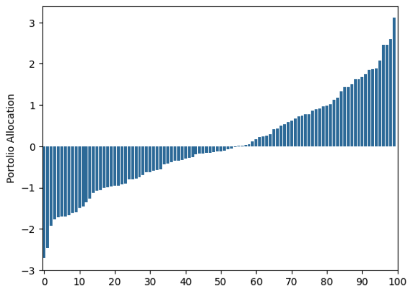
As you can see, this allocation is far from the equal weights allocation. If we had 100 dollars to invest we should allocate 1 dollar in each of the assests. This allocation is telling us we some times have to allocate 300 dollars to some of the assets!

Let’s look at the allocation when we use 100 years of data:

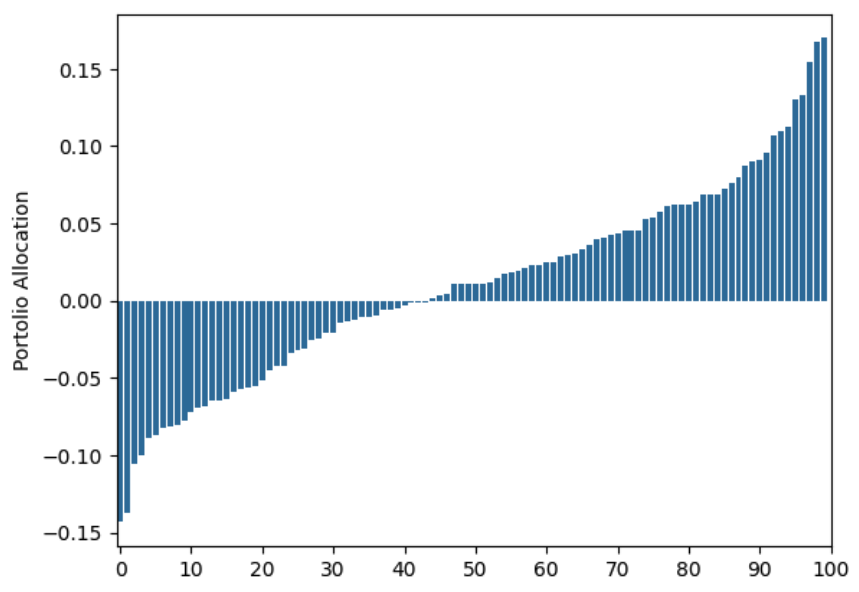
Still very far from the uniform allocation.

With 1,000 years of data:

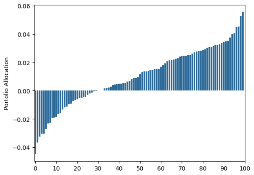
Still off. With 25,000 years of data:

Ok, it’s finally starting to get there. We only had to wait 25,000 years…

You may argue that the portfolio allocation does not need to be close to the optimal, in order for the allocation to achieve similar performance. That is, we don’t really care that our allocations are off if they guarantee close to the same returns as the uniform allocation. So let’s plot the wealth trajectories of the allocations we just found:

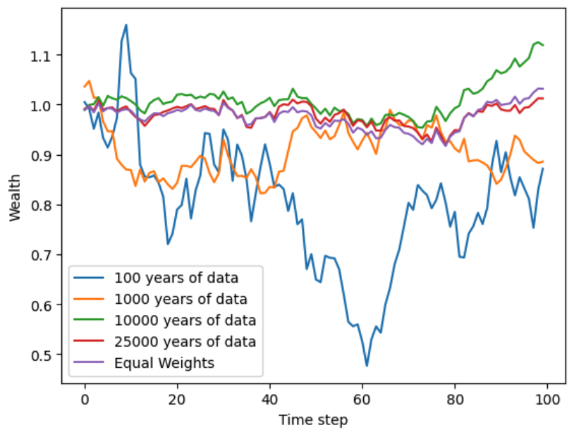
For an allocation to be good, it should be following the “equal weights” trajectory, as you can see this only starts happenning when we use more that 10,000 years worth of data.

We need so many samples to start building reasonable portfolios!

The Source of Error

Why are the allocations so bad? Where is the error coming from? If you plug in the true covariance matrix and use only 4 years of data, you get a similar allocation than if you use 25,000 years and estimatate the returns and covariance matrix:

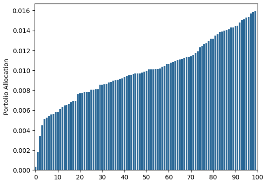
So you may think that the misallocation comes from our noisy covariance estimate. But if we plug in the true expected returns and the estimated covariance matrix you get a very similar allocation:

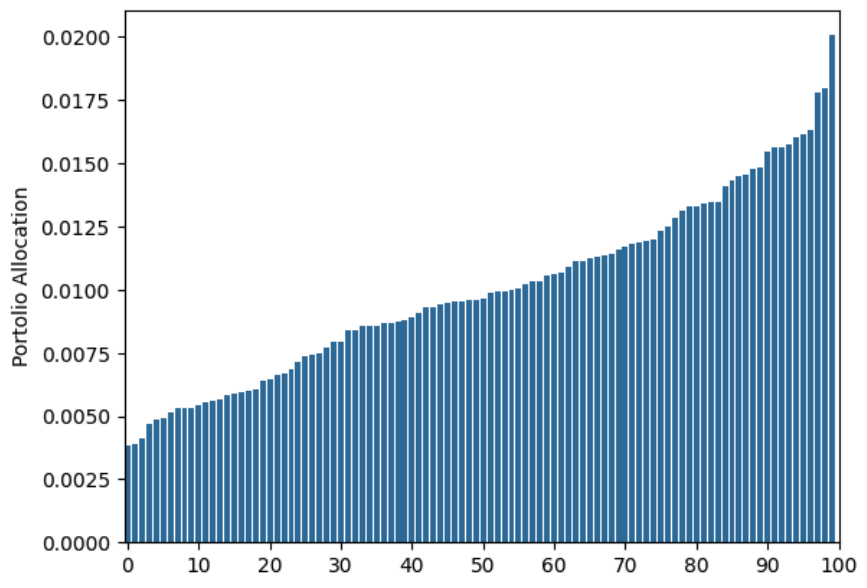
So, you really need accuate estimates for both the expected returns and the covarainace matrix for the mean variance portfolio to be good.

Final Thoughts

These simulations show one of the big caveats of mean variance portfolios – they are very sensitive to the input expected rewards and covariance matrix. Over estimating some returns may result in highly concentrated portfolios. To make things worse, in these simulations we used the Gaussian distribution to model returns, in the real world you will encounter fait tails which will only make these issues worse.

Disclaimer: The content provided on this blog is for educational purposes only and is not intended to be financial advice. The views and opinions expressed here are solely those of the authors and should not be construed as professional financial advice. Readers are encouraged to consult with a qualified financial advisor before making any financial decisions based on the information provided on this blog.