In this post we study how to trap a set of points in high dimensions inside an ellipsoid with minimal volume (John, 1948). This problem has applications in statistics and outlier detection, but my motivation for studying this problem is to be able to represent “uncertainty sets” for doing Robust Optimization. Please see this post if the terms “uncertainty sets” and Robust Optimization are new to you, if all you care is about learning geometry and optimization just keep reading.

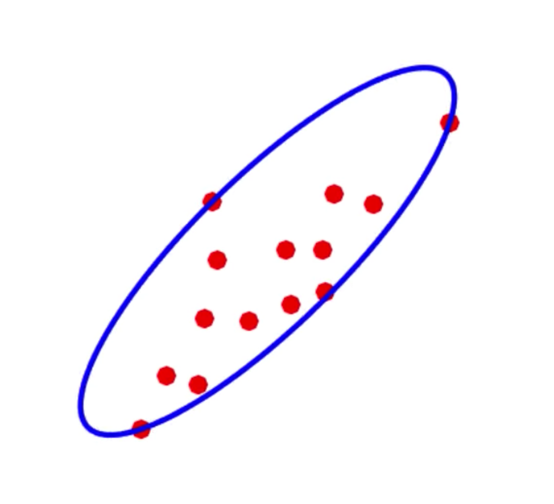
Pictorially, what I’m trying to do is, find a description of the ellipsoid shown in the picture below.

This post is organized as follows, first I will show how to concisely represent/describe ellipsoids using matrices, then I’ll present an alternative parametrization of ellipsoids that is useful for entering the problem into a solver. Finally I will pose the Minimal Volume Enclosing Ellipsoid (MVEE) problem as a convex optimization problem.

A Primer On Ellipsoids

Before we discuss ellipsoids lets get comfortable describing their simplest form, unit balls. You probably remember from school that in two dimensions the ball of radius 1, can be represented as the set of all points $x_1, x_2$ such that

$x_1^2 + x_2^2 \leq 1.$

That is the two-dimensional unit ball is $\mathcal{B}_2 = \lbrace x_1, x_2 \in \mathbb{R}: x_1^2 + x_2^2 \leq 1 \rbrace$. In $n$ dimensions, we have

$x_1^2 + x_2^2+ ... + x_n^2 \leq 1.$

It is annoying to work with these large equations so, if $x \in \mathbb{R}^n$ is is the column vector with entries $x_1, x_2, …, x_n$ we can simply write $\mathcal{B}_n = \lbrace x \in \mathbb{R}^n: x^\top x \leq 1 \rbrace$.

Great, now, to go from a unit ball to an ellipsoid (lets focus on ellipsoids centered around the origin) all we have to do is “squish it” and rotate it. A great way to represent, squishing and rotating a set of points is through applying linear functions of the form $f(x) = Ax$ where $A$ is an $n$ by $n$ matrix. For example, imagine applying pressure to the top of the unit ball so it no longer reaches 1 but instead it only reaches .5 (keeping its width constant), and then rotating counterclockwise 45 degrees. This transformation is equivalent to first sending the unit vector pointing upwards from $[0; 1]$ to $[0; .5]$, then the 45 degree rotation sends $[1; 0] \rightarrow [\frac{1}{\sqrt{2}}; \frac{1}{\sqrt{2}}]$ and $[0; .5] \rightarrow [-\frac{1}{2\sqrt{2}} ; \frac{1}{2\sqrt{2}}]$. The matrix that represents this transformation is

$A = \begin{bmatrix} \frac{1}{\sqrt{2}} & -\frac{1}{2\sqrt{2}} \\ \frac{1}{\sqrt{2}} & \frac{1}{2\sqrt{2}} \end{bmatrix}.$

That’s right, the first column of the matrix tells you where the unit vector $[1; 0]$ gets mapped to, and the second column tells you where the other unit vector $[0; 1]$ gets mapped to. The previous is not a coincidence, by the way, if you feel like digging deeper into why this is true I highly recommend this post from Gregory Gundersen’s blog, which I’ve obviously drawn inspiration (and template files (with his permission)) from.

So, our ellipse $\mathcal{E}$ is the set of all points $y$ such that $y = Ax$ where $x$ is in the unit ball. Since we are interested in “full dimensional” ellipsoids in $\mathbb{R}^n$, that is we are not interested in representing a 2-d circle in 3-d space, the matrix $A$ is assumed to be invertible. More formally our ellipsoid is

$\mathcal{E} = \lbrace y \in \mathbb{R}^n, \exists x \mathbb{R}^n: y = Ax, x^\top x \leq 1 \rbrace.$

Since A is invertible we have

$x = A^{-1} y \tag{1}$

so that

$\mathcal{E} = \lbrace y \in \mathbb{R}^n: y^\top A^{-\top}A^{-1} y \leq 1 \rbrace.$

Back to our numerical example, computing $A^{-\top}A^{-1}$ we get $B = \frac{1}{2}[[5, -3];[-3, 5]]$, so that $x^\top A^{-\top}A^{-1} x = \frac{5}{2}(x^2+y^2) - 3xy$ and this is what the ellipsoid looks like:

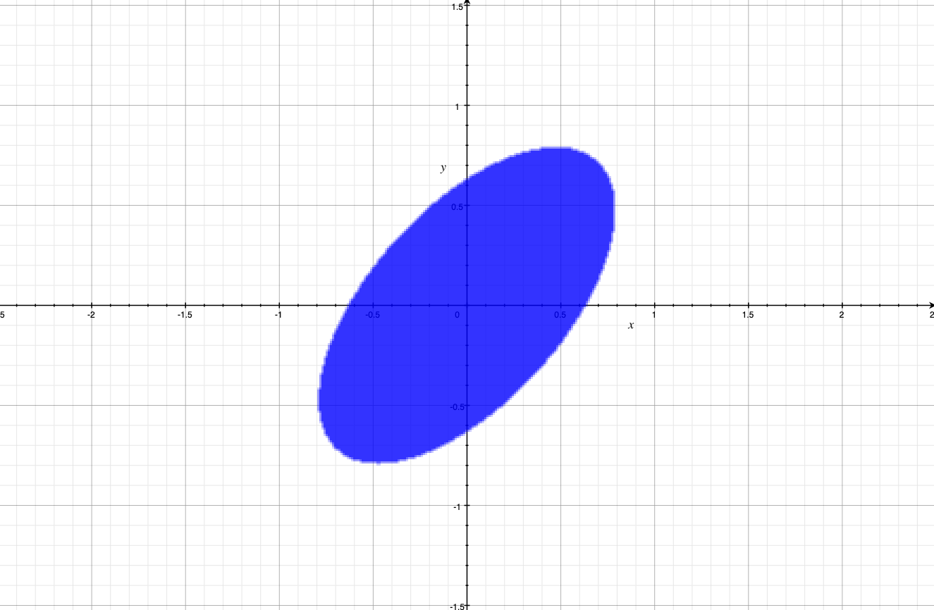
just like we designed it; squished at the top, then rotated 45 degrees counter-clockwise.

It is common in the literature to see $n$-dimensional ellipsoids parametrized with a symmetric positive-semidefinite (I’ll explain in a sec) matrix $B\in \mathbb{R}^{n\times n}$ via

$\mathcal{E} = \lbrace x \in \mathbb{R}^n: x^\top B x \leq 1 \rbrace.$

So, if we ever encounter a parametrization of this kind we know that if we can factorize $B$ as

$B = A^{-\top} A^{-1}, \tag{2}$

then $A$ tells us how a unit ball is being transformed to create the ellipsoid. Intuitively, a matrix $B$ is positive-semidefinite (PSD) if there exists a decomposition of the form $B = A^{-\top} A^{-1}$ where A squishes and/or rotates but does not collapse dimensions. Now, what if we don’t want our ellipsoids to be centered at $0$, what if we want them centered at $b\in \mathbb{R}^n$? All we have to do is:

$\mathcal{E} = \lbrace x \in \mathbb{R}^n: (x-b)^\top B (x-b) \leq 1 \rbrace \tag{3}.$

To see why this is true think that if before the translation of the ellipsoid you had a point inside it: $\bar{x}$ (and thus it satisfied $\bar{x}^\top B \bar{x} \leq 1$), after translation you have to plug in $\bar{x} + b$ to get $(\bar{x} + b - b)^\top B (\bar{x} + b - b) = \bar{x}^\top B \bar{x} \leq 1$.

An Alternative Parametrization Of Ellipsoids

Another way to parametrize an ellipsoid is via a PSD matrix $C \in \mathbb{R}^{n\times n}$ and a vector $c \in \mathbb{R}^n$. The parametrization is all $x\in \mathbb{R}^n$ such that:

$\Vert C x + c\Vert_2^2 \leq 1.$

How does this parametrization relate to the one in (3)? Lets expand:

\begin{align} \Vert C x + c\Vert_2^2 & = (C x + c)^\top (C x + c) \cr & = x^\top C^\top C x + 2 x^\top C^\top c + c^\top c. \end{align}

Expanding (3) we get

\begin{align} (x-b)^\top B (x-b) = x^\top B x - 2x^\top B b + b^\top b, \end{align}

it must follow that if we are referring to same elipsoid with two different representations the following must hold: $B = C^\top C$, and $C c = b$. More importantly, because of (2) it must hold that

\begin{align} C = A^{-1} \tag{4}. \end{align}

Why equation (4) is important will be explained in a minute.

Minimal Volume Ellipsoid

Recall the problem we are trying to solve. We have been given a set of $N$ points $x_1, x_2, …, x_N$ in $\mathbb{R}^n$ and we want to find the ellipsoid of smallest volume that contains it. Using our second parametrization of ellipsoids, we know that we are looking for $C$ in the set of all PSD matrices and $c \in \mathbb{R}^n$ such that:

$\Vert C x_n + c\Vert_2^2 \leq 1 \qquad \forall n \in [N].$

But how do express that we want the ellipsoid of smallest volume? The trick is to remember from linear algebra that the determinant of a matrix is proportional to how the linear transformation increases/decreases volume. Remember how two sections ago we were thinking about creating ellipsoids by squishing and rotating unit balls by applying the mapping $A$? We want to minimize $\det(A^{-1})$, but how are $C$ and $A$ related? Well, we established this relation in equation (4). So our problem formulation is:

\begin{align} \min_{C, c} \quad & \det(C^{-1}) \cr & \Vert C x_n + c\Vert_2^2 \leq 1 \qquad \forall n \in [N]. \end{align}

We have a formulation for the MVEE optimization problem, but is this problem convex? Do there exist algorithms to efficiently solve this problem? The answer to the first question is no, this is because $\det(\cdot)$ is neither convex nor concave over the set of PSD matrices (see F_G’s answer). But we are in luck, because $\log(\det(\cdot))$ is concave. So. if we modify our objective function to be $\log(\det(C^{-1})) = \log(\frac{1}{\det(C)}) = - \log(\det(C))$, we are minimizing a convex function! To conclude that the whole optimization problem is a convex one we would have to show two more things, that the set of PSD matrices is convex, and that each of the sets $\lbrace C : \Vert C x_n + c\Vert_2^2 \leq 1 \rbrace$ is convex. Turns out both statements are true, unfortunately I won’t prove them right now because I want to focus on trying to build robust portfolios. But if you want to learn how to prove this I recommend these lecture notes on Semidefinite Programming or Ch. 8 from (Boyd & Vandenberghe, 2004).

Final Thoughts

To summarize, the MVEE can be formulated as the following (convex) Semidefinite Program

\begin{align} \min_{C, c} \quad & - \log(\det(C)) \cr & \Vert C x_n + c\Vert_2^2 \leq 1 \qquad \forall n \in [N]. \end{align}

This formulation is useful because there exist general purpose algorithms for solving these kinds of problems. In the next post I will show how given samples of asset returns (these will be the points $\lbrace x_n \rbrace$) we can use a MVEE to find uncertainty sets which we can then incorporate into our robust formulation of the mean-variance portfolio problem.