In a previous post we explored what happens when we try to build Mean Variance (also known as Markowitz) Portfolios using a finite number of samples from the distribution of returns. The results were discouraging, unless you have a prohibitively large number of samples, the resulting portfolios will be very far from the optimal one. In this post, we explore whether the Robust Optimization framework can address these issues.

Review of Mean Variance Portfolios

Before introducing Robust Optimization let’s review the problem we want to solve. We are faced with the problem of allocating our wealth across a number of assets but we are uncertain about what their returns are going to be. If the asset returns were Gaussian with mean $\mu$ and covariance matrix $\Sigma$, then allocating our wealth according to the solution of the mean-variance portfolio (MVP) problem

\begin{align} \max_{w} \thinspace & \mu^\top w - \frac{1}{2} w^\top \Sigma w \cr s. t.\thinspace &1^\top w = 1, \tag{1} \end{align}

would guarantee that (asymptotically) our wealth would grow exponentially quickly and at the fastest possible rate. If you are used to seeing $\lambda$ instead of $\frac{1}{2}$ in the objective please review this post.

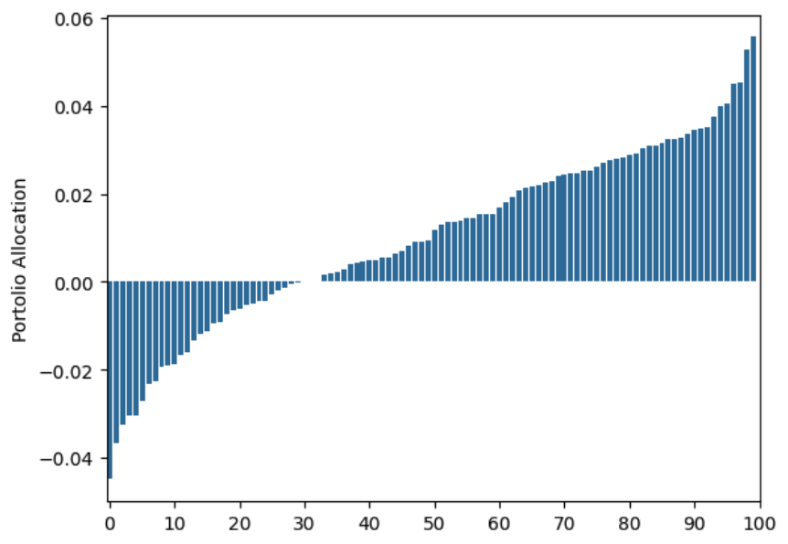
In practice, we don’t have knowledge of $\mu$ and $\Sigma$, so typically, we would estimate them and then plug the estimates $\hat{\mu}, \hat{\Sigma}$ into (1). Previously we saw how even with 1,000 years worth of daily returns the MVP would produce terrible portfolios. As a reminder, the simulation consisted of 100 assets, all of them with independent and identically distributed return distributions, for which the optimal portfolio consists of allocating $\frac{1}{100}$ of your wealth on each asset. Instead this is the allocation Markowitz produced:

If you think about it, we were being wasteful with our samples. We were estimating $\hat{\mu}, \hat{\Sigma}$ but using only their point estimates; with all the samples we could compute confidence intervals of each of these quantifies and somehow try to modify the optimization problem so that it takes this information into account. This is exactly the idea we will explore in the rest of this post.

Robust Optimization

Robust Optimization (RO) (Ben-Tal et al., 2009) is a worst case approach to modeling optimization problems where there is uncertainty in the parameters of the problem (in our example we are uncertain about $\mu$ and $\Sigma$). In the RO framework we must specify an “uncertainty set” for our parameters, that is, we must specify a set $\mathcal{U}$ in which we think that the true problem parameters $\mu, \Sigma$ live. The robust formulation of the MVP will be:

\begin{align} \max_{w} \min_{(\mu, \Sigma)\in \mathcal{U}} \thinspace & \mu^\top w - \frac{1}{2} w^\top \Sigma w \cr s. t.\thinspace &1^\top w = 1, \tag{2} \end{align}

What the above formulation says is that we must pick a portfolio $w$ knowing that and adversary is going to try to hurt us by picking the worst possible return vector $\mu$ and covariance matrix $\Sigma$ in the uncertainty set $\mathcal{U}$. As I mentioned earlier this is a worst case approach to handling uncertainty, but in the context of finance I think it’s reasonable, we better be safe than sorry.

Modeling The Uncertainty

To apply the framework of RO to portfolio construction we must specify the uncertainty set $\mathcal{U}$. The following specification of the uncertainty set comes from (Boyd et al., 2017). I must say, I don’t love the specification and I think modeling the uncertainty via ellipsoids will be better but I’ll explore that in another post since I thought it’d be important to understand Boyd et al’s specification first.

$\mathcal{U}$ will be such that the expected return of asset $i$, $\mu_i$ lives inside a box. We set $\mu_i = \bar{\mu}_i + \delta_i$ with $\delta_i \leq \vert \rho_i \vert$ where $\bar{\mu}_i$, $\rho_i$ are real values specified by us. The uncertainty in the covariance matrix will be modeled as $\Sigma = \bar{\Sigma} + \Delta$ where $\bar{\Sigma}$ is the “nominal” covariance matrix and $\Delta$ is a symmetric matrix satisying

\begin{align} \Delta_{ij} \leq \kappa \vert \bar{\Sigma_{ii}} \bar{\Sigma_{jj}}\vert. \tag{3} \end{align}

With this uncertainty model, we must provide actual values for $\mu, \rho \in \mathbb{R}^n$, $\bar{\Sigma}, \Delta \in \mathbb{R}^{n\times n}$. In the rest of this post I will refer to entries of a covariance matrix $\Sigma$ as $\sigma_{ij}$ when $i \neq j$ and as $\sigma^2_i$ when $i=j$.

Before we attempt to go back to (2) and try to solve it using our model for $\mathcal{U}$, let’s examine the intuition behind (3). Equation (3) implies that

$\bar{\sigma}_{ij} - \kappa \bar{\sigma}^2_{ii} \bar{\sigma}^2_{jj} \leq \sigma_{ij} \leq \bar{\sigma}_{ij} + \kappa \bar{\sigma}^2_{ii} \bar{\sigma}^2_{jj} \tag{4}$

So that when $i = j$, we have

$\bar{\sigma}^2_{ii} (1 - \kappa) \leq \sigma^2_{ij} \leq \bar{\sigma}^2_{ii} (1 + \kappa),$

this means that in our uncertainty model we allow for misspecifying all variances by at most a factor of $\kappa$. When $i \neq j$ the consequence is that the (almost) correlation is bounded by an additive factor of $\kappa$, that is

$\vert \frac{\sigma^2_{ij}}{\bar{\sigma}_{ii}\bar{\sigma}_{jj}}\vert \leq \bar{\rho}_{i,j} + \kappa,$

where $\bar{\rho_{i,j}}$ is the correlation coefficient computed from $\bar{\Sigma}$. Hopefully this gives you a better intuition of what (3) implies.

You should be wondering, why is a single $\kappa$ value allowed? What if we were more confident about the variances of some assets vs others? Could we have a $\kappa_{i,j}$ for every $i,j$ pair?

The Robust Counterpart of Mean-Variance Portfolios

We turn our attention back to the minimax problem

\begin{align} \max_{w} \min_{(\mu, \Sigma)\in \mathcal{U}} \thinspace & \mu^\top w - \frac{1}{2} w^\top \Sigma w \cr s. t.\thinspace &1^\top w = 1 \end{align}

but this time with the uncertainty set that we defined in the previous section

$\mathcal{U} = \{(\mu, \Sigma): \exists \delta \in \mathbb{R}^n, \Delta \in \mathbb{R}^{n \times n}: \mu = \hat{\mu} + \delta, \Sigma = \bar{\Sigma} + \Delta, \vert \delta \vert \leq \rho, \Delta_{ij} \leq \kappa \vert \bar{\Sigma_{ii}} \bar{\Sigma_{jj}}\vert\}.$

As we will see shortly, the inner problem admits a closed form expression for its solution, so we will be able to find a robust portfolio by a solving convex problem instead of a minimax game! This means we don’t have to pay a computational complexity cost for solving the robust version of the problem! This situation does not happen in general, but in this case the uncertainty set was designed so that this would happen.

Let us now solve

\begin{align} \min_{(\mu, \Sigma)\in \mathcal{U}} \thinspace & \mu^\top w - \frac{1}{2} w^\top \Sigma w. \end{align}

Notice that the problem decouples so we can first minimize the first term by finding the worst $\mu$ in the uncertainty set and independently, we can find the $\Sigma$ that maximizes (note the minus sign) $w^\top \Sigma w$. For the first term we have

\begin{align} &\min_{\mu\in \mathcal{U}} \thinspace \mu^\top w \cr &= \min_{\mu\in \mathcal{U}} \thinspace (\bar{\mu} + \delta)^\top w \cr &= \min_{\vert \delta_i\vert \leq \rho_i} (\bar{\mu} + \delta)^\top w \cr &= \min_{\vert \delta_i\vert \leq \rho_i} \bar{\mu}^\top w + \delta^\top w \cr &= \bar{\mu}^\top w - \sum_{i\in[n]} \rho_i \vert w_i \vert \tag{5}. \end{align}

The last equality is true because if we asign a positive weight for $w_i$ the adversary picks $\delta_i = -\rho_i$ and if the weight for $w_i$ is negative, the adversary can pick $\delta_i = \rho_i$. So regardless of the sign of our portfolio weight the adversary damages us with $-\rho_i \vert w_i \vert$. Before we move on, notice that Eq. (5) is the usual mean return of the portfolio $\bar{\mu}^\top w$ but now we have a regularization term where we get penalized by how uncertain we are about the asset returns.

Let’s now examine the variance term:

$\max_{\Sigma\in \mathcal{U}} \thinspace w^\top \Sigma w = w^\top \bar{\Sigma} w + \max_{\vert \Delta_{ij} \vert \leq \kappa \bar{\sigma}^2_{ii} \bar{\sigma}^2_{jj}} \thinspace w^\top \Delta w$

and focus on the $\max$. Expanding $w^\top \Delta w$ we have that

$\max_{\vert \Delta_{ij} \vert \leq \kappa \bar{\sigma}^2_{ii} \bar{\sigma}^2_{jj}} \thinspace w^\top \Delta w \\ = \max_{\vert \Delta_{ij} \vert \leq \kappa \bar{\sigma}^2_{ii} \bar{\sigma}^2_{jj}} \sum_{i,j \in [n]} w_i w_j \Delta_{ij} \\ = \sum_{i,j \in [n]} \vert w_i w_j \vert \kappa \bar{\sigma}^2_{ii} \bar{\sigma}^2_{jj} \\ = \kappa \sum_{i,j \in [n]} \vert w_i\vert \vert w_j \vert \bar{\sigma}^2_{ii} \bar{\sigma}^2_{jj} \\ = \kappa (\sum_{i \in [n]} \vert w_i \vert \bar{\sigma}^2_{ii})^2$

Where the second equality follows by the same reasoning we used for Eq. (5). Before we move on, can you see why we cannot use a $\kappa_{ij}$ in our uncertainty set and must use a single $\kappa$? The answer is that we wouldn’t be able to factor it out in the second to last line and that function would not necesarily be convex.

We are done, we have successfully reformulated the minimax game (2) into the following convex problem

\begin{align} \max_{w} \thinspace & \bar{\mu}^\top w - \sum_{i\in[n]} \rho_i \vert w_i \vert - \frac{1}{2} w^\top \hat{\Sigma} w - \frac{1}{2}\kappa (\sum_{i \in [n]} \vert w_i \vert \bar{\sigma}^2_{ii})^2 \cr s. t.\thinspace &1^\top w = 1. \tag{6} \end{align}

It is now time to test the quality of these Robust Markowitz Portfolios (RMP).

Simulations

Setup

We will use the same simulation setup we used in the previous post. As a reminder, there are 100 assets, all of them with Gaussian returns with mean zero and standard deviation equal to .1, all returns are independent from each other. If we were to have acess to the true vector of expected returns $\mu$ and the true covariance matix $\Sigma$, the optimal portfolio according to (1) is the uniform allocation, that is, allocate 1% of our wealth to every asset.

In real life we don’t have access to $\mu$ and $\Sigma$ so in the rest of this post we explore how to build portfolios using only daily samples from the distribution of returns. The most straightforward thing to do given a finite number of samples is to create estimates $\hat{\mu}, \hat{\Sigma}$ and plug them into (1). Unfortunately, as shown in this previous post even with thousands of years worth of data the resulting portfolios were very far from the optimal allocation and performed poorly.

Notice, that we were being wasteful, we were only creating point estimates for $\hat{\mu}$ and $\hat{\Sigma}$ when we could have actually built confidence intervals for $\mu$ and $\Sigma$ and somehow try to incorporate them into (1). Back then we didn’t have the framework of Robust Optimization so incorporating the uncertainty into the problem wasn’t traightforward. But now we do, all we have to do is use our samples to come up with values for $\rho, \bar{\mu}, \bar{\Sigma}$ and $\kappa$ and then just plug them into our robust version of the mean-variance portfolio (6). We will estimate these parameters using the bootstrap.

Using the Bootstrap to Build Uncertainty Sets

There are probably many ways to come up with values for $\rho, \bar{\mu}, \bar{\Sigma}$ and $\kappa$. In this post we will use the bootstrap (creating “new” datasets by sampling, with replacement, from the samples we are given) to come up with values for $\rho, \bar{\mu}, \bar{\Sigma}$ and $\kappa$. I did not see the results change too much once I started using more than 1000 bootstrap samples, so I will not discuss this point further. We set $\bar{\mu}_i = \frac{\mu_i^{min} + \mu_i^{max}}{2}$ for every asset $i \in [n]$ where $\mu_i^{min}$ is the smallest expected return using the bootstrap samples, $\mu_i^{max}$ is defined similarly. Additionally, we set $\rho_i = \frac{\mu_i^{max} - \mu_i^{min}}{2}$ and let $\bar{\Sigma}$ be the sample covariance matrix. Finally,

$\kappa = max_{i,j\in[n], k} \vert \frac{\sigma^2_{ijk} - \bar{\sigma}^2_{ij}}{\bar{\sigma}^2_{ii}\bar{\sigma}^2_{jj}}\vert$

where $\sigma^2_{ijk}$ is the $ij$-th entry of the sample covariance matrix that uses the $k$-th bootstrap sample. For more details on the simulations please see the Github repo.

Simulation Results

Using daily observations of returns for one year and building the Robust Markowitz Portfolio this is the allocation we get:

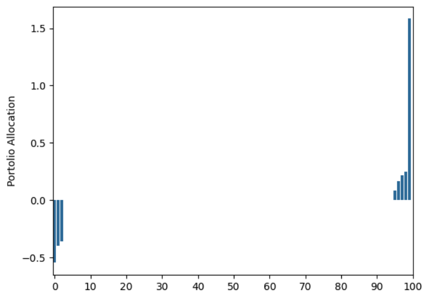
The allocation is telling us to go short a few stocks (some with ~50% of our initial wealth), and to long a few other ones using leverage. This allocation is clearly very different from the optimal (uniform) allocation that has access to the true values of $\mu$ and $\Sigma$. A somewhat interesting phenomenon is that the way we accounted for uncertainty in the expected returns lead us to add $- \sum_{i\in[n]} \rho_i \vert w_i \vert$ to the objective, this $l$-1 norm is inducing sparcity into the portfolio forcing us to not allocate any capital to ~90% of the assets.

The above robust portfolio is bad, does it get better if we use daily returns for a longer time period? Unfortunately, that does not seem to be the case. Here is the allocation using 10,000 years worth of data:

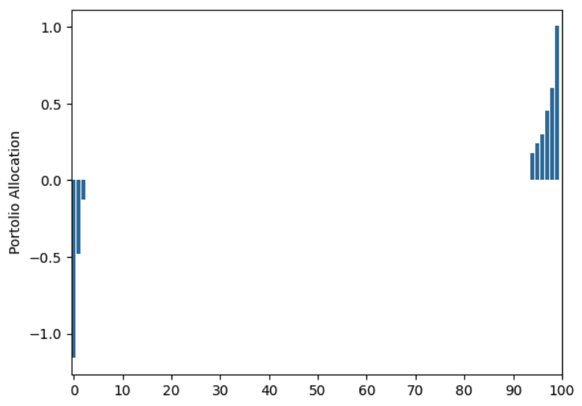
Sadly, no noticeable improvements at all from using Robust Optimization…

Final Thoughts

Unfortunately, it looks like using Robust Optimization and the uncertainty sets from (Boyd et al., 2017) do not yield a much better approach to building portfolios than the original formulation. But we should not be discouraged by this, at least we know we shouldn’t use this techique in the real world!

Before wrapping up, I have to say that I still have some hope at making Mean Variance portfolios work – I think that using ellipsoids to represent the uncertainty set is an idea worth trying. The reason for this is that with ellipsoids we can capture relationships in the uncertainty that we can not capture with “boxes” like we did in this post, moreover the $l$-1 penalty which induces sparsity will probably disappear. We will explore this idea in detail in a future post.

Disclaimer: The content provided on this blog is for educational purposes only and is not intended to be financial advice. The views and opinions expressed here are solely those of the authors and should not be construed as professional financial advice. Readers are encouraged to consult with a qualified financial advisor before making any financial decisions based on the information provided on this blog.