A Brief Review of The Sharpe Ratio

The Sharpe ratio (Sharpe, 1966) is a metric traders and portfolio managers use to measure their performance. At a high level, the ratio quantifies the expected returns of a strategy per unit of “risk”. Here “risk” will be measured using the square root of the variance of the returns, sometimes also called “volatility”. There are two flavors of it, the ex-post Sharpe ratio:

\begin{align} S = \frac{ \hat{r} - r_{free}}{\sqrt{\hat{\sigma}^2}}, \end{align}

where $\hat{r} = \frac{1}{N} \sum_{i=1}^N r_i$ is the sample mean of your strategies’ realized daily returns $r_1, …, r_N$, $\hat{\sigma}^2 = \frac{1}{N} \sum_{i=1}^N (r_i - \hat{r})^2$ is the sample variance, and $r_{free}$ is the risk free rate. Similarly, the ex-ante Sharpe ratio is defined as:

\begin{align} S = \frac{\mathbb{E}[r] - r_{free}}{\sqrt{\mathbb{V}[r]}}, \end{align}

where $r$ is the random variable representing the return of your strategy, $\mathbb{E}[r]$ is the expected return of your strategy, and $\mathbb{V}[r]$ is the variance.

If you are a trader, your boss may use the ex-post version to measure your past performance, so if you know you will be judged by the ex-post version you may want to find a strategy to maximize the ex-ante version.

First Thoughts

A few things jump to mind about the definition of Sharpe ratio. The first one is that measuring “risk” with the standard deviation is not great because it penalizes large gains. The second one is that there may be trading strategies that have extremely high ratios, until they don’t. For example someone selling naked out of the money options will consistently be receiving a steady “income” until they blow up. Up until the point they blow up, the ex post will be high. The last thing that jumps to me is: why use the (arithmetic) mean return as the numerator when you could be using the (geometric) mean return? This will most likely prevent us from accumulating wealth in the long run.

Organization of This Post

The rest of this post has three sections. The first section shows why people think this quantity is a good metric for measuring performance. The second section shows how to build a portfolio that maximizes this metric by transforming a non-convex problem into a convex one. The second section also shows how this portfolio accumulates wealth in the long run (spoiler alert, it’s not as good as the Kelly portfolio). In the last section (my favorite) I show how it is possible to have strategies with the same Sharpe ratio where some grow your wealth at an exponential rate and others lead you straight to ruin. As usual, you can find the code for this post on Github.

Using The Sharpe Ratio To Pick Between Strategies

Let’s assume we have two good assets to allocate money on. Asset 1 has expected return $\mu_1 = .05$ and std. deviation $\sigma_1 = .1$, asset 2 has $\mu_2 = .04$ and $\sigma_2 = .05$, both asset’ returns are normally distributed. So, asset 1 has higher expected returns compared to asset 2 but it also has a larger variance. Assuming the risk free rate is equal to 0, the Sharpe ratios are $S_1 = \frac{.05}{.1} = .5$ and $S_2 = \frac{.04}{.05} = .8$. So, asset 2 seems to be a better risk adjusted return.

Imagine your portfolio’s initial dollar value is 1, it is allowed to have at most .1 units of risk (measured by its volatility), and you have access to leverage. If this is the case you can borrow another dollar and invest two dollars on asset 2 (let’s call this strategy 2), your portfolio will have volatility equal to $2 *\sigma_2 = .1$ but its expected return will be $2 * .04 = .08$, which is greater than if you just invested your unit of wealth on asset 1 (remember you maxed out your risk so you can borrow). Let strategy 1 be investing your dollar into asset 1.

Now, truth is, you and I do not get paid in “Sharpe ratio units”, we get paid in dollars. You should be wondering, how does the Sharpe ratio translate into actual money? If we lock our money into these strategies for 2000 rounds, this is what our log wealth would look like:

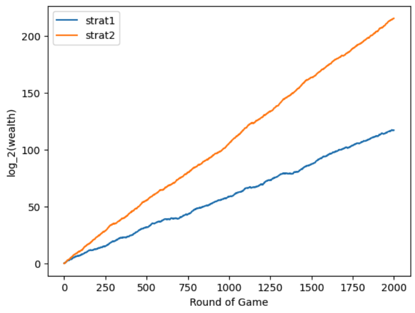
In this situation, the Sharpe ratio seems to be doing something useful.

A reasonable question is: can we do better than by just leveraging and investing everything in asset #2? If you’ve read my previous post on portfolio optimization you may be wondering what happens when we build a portfolio that maximizes expcected log wealth (the Kelly portfolio) and has volatility equal to .1. In this particular example, to find the Kelly portfolio we can just solve the following convex problem

\begin{align} \max_{w} \thinspace & \mu^\top w - \frac{1}{2} w^\top \Sigma w, \cr s. t.\thinspace & w^\top \Sigma w \leq \sigma_{allowed}^2, \end{align}

with the appropriate parameters. If you don’t remember why this objective is a good approximation to maximizing log wealth please review this previous post.

Assuming our two assets are uncorrelated we get that we should invest 53% of our wealth on asset 1 and 170% of our wealth on asset 2 (remember we are allowed to take on leverage as long as the volatility of our portfolio is less than .1). This is what our log wealth would look like for the three strategies we just discussed:

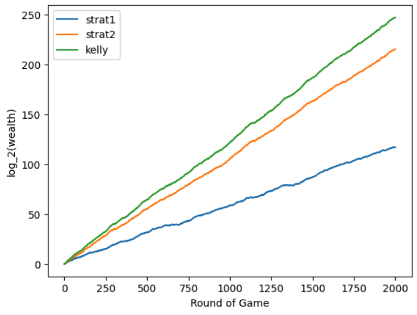
So, the Kelly portfolio seems to be a good idea. Moreover, the Sharpe ratio for the Kelly portfolio is $\approx 0.96$ which is greater that the $.8$ from strategy #2.

The Sharpe ratio seems to be useful, and it looks like it correlates with making more money. But is this relationship actually true? Does maximizing the (ex-ante) Sharpe ratio guarantee we are maximizing our wealth in the long run? We answer this question negatively in the next section.

The Sharpe Ratio Maximizing Portfolio

We are interested in the properties of the portfolio that is the solution to the following (nonconvex) optimization problem

\begin{align} \max_{w} \thinspace & \frac{\mu^\top w}{w^\top \Sigma w} \cr s. t.\thinspace & 1^\top w = 1. \tag{1} \end{align}

In particular, we want to know whether it maximizes long term wealth (i.e. it is equivalent to the Kelly portfolio or not). At first glance we have a problem because the objective is nonconvex, the good news is that we can translate it into a convex problem.

The (Convex) Equivalent Problem for Finding the Maximum Sharpe Ratio Portfolio

This trick comes from Theo Diamanis’ blog post. Multiply the numerator of the objective function by any $\alpha > 0$ (this changes the objective value but not the optimal solution), then we add the constraint $\mu^\top \alpha w = 1$ and the objective becomes $\max \frac{1}{w^\top \Sigma w}$, but this is equivalent to $\min w^\top \Sigma w$. We have transformed our problem to:

\begin{align} \min_{w} \thinspace & w^\top \Sigma w \cr s. t. \thinspace & 1^\top w = 1 \cr & \mu^\top \alpha w = 1 \end{align}

Changing to decision variables $y = \alpha w$, this problem is equivalent to

\begin{align} \min_{w} \thinspace & y^\top \Sigma y \cr s. t. \thinspace & 1^\top (\frac{1}{\alpha} y) = 1 \cr & \mu^\top y = 1. \end{align}

Now, notice that $1^\top (\frac{1}{\alpha} y) = 1$ is equivalent to $1^\top y = \alpha$, and we haven’t picked a specific value for $\alpha$. So, if we set $\alpha = 1^\top y$, the constraint becomes $1^\top y = 1^\top y$, which is redundant, so we don’t need to include it in the formulation of the problem. We are done, to solve (1) all we need to do is to solve the following convex problem

\begin{align} \min_{w} \thinspace & y^\top \Sigma y \cr s. t. \thinspace & \mu^\top y = 1. \end{align}

to get $y_{opt}$, and then set $w_{sharpe} = \frac{y_{opt}}{1^\top y_{opt}}$.

Is Maximizing the Sharpe Ratio Best For Long Term Wealth?

In our specific example, the Kelly portfolio will invest 100% of its wealth on asset 1 since it has higher expected returns and its variance is not large enough to wipe us out, its Sharpe ratio is around 0.46 and compounds around .0414% per period. The maximum sharpe ratio portfolio invests 24% on asset 1 and 76% on asset 2, its sharpe ratio is 0.95 and it compounds around .0412% per period. With this we conclude that maximizing Sharpe ratio is not the best receipe maximizing for long run wealth.

The Sharpe Ratio Can be The Same For Winning and Losing Strategies

Let’s examine the Sharpe ratios of three strategies in our favorite coin betting game. The set up of the game is that there is a coin which turns up heads with probability .6 and tails with probability .4, you are allowed to wager as much of your wealth as you want on the outcome of the coin. If the coin turns out heads you double your money, and if it comes out tails you lose it all. What fraction of your wealth do you bet on heads coming out in each round?

As we saw in the previous post, the optimal strategy to maximize wealth in the long run is to bet 20% of your wealth in every round of the game, this strategy is called full-Kelly. If we bet 10% (half-Kelly) our wealth will also grow at an exponential rate, albeit a smaller rate. If we bet anything more than 38% our our wealth in every round we, will go bust. These is what some wealth trajectories may look like:

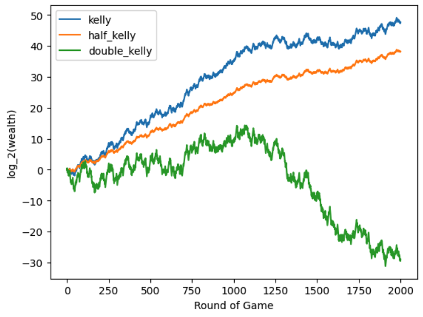
So what do the Sharpe ratios look like for these three different strategies? Full Kelly: .02, Half Kelly: .02, Double Kelly: .02. What!?! To see why this happens let’s look at the returns of Kelly, they will look something like: .2, .2, -.2, .2, -.2, along the same trajectory those for half Kelly will look like .1, .1, -.1, .1, -.1, and something similar for double Kelly. So, for one strategy the returns are just a scaled version of one of the other strategies. When $r_{free}=0$, plugging $r’=a r$ into the definition of Sharpe ratio we get

\begin{align} \frac{\mathbb{E}[ar] }{\sqrt{\mathbb{V}[ar]}} &= \frac{a\mathbb{E}[r]}{\sqrt{a^2\mathbb{V}[r]}} \cr &= \frac{a\mathbb{E}[r] }{a\sqrt{\mathbb{V}[r]}} \cr &= \frac{\mathbb{E}[r]}{\sqrt{\mathbb{V}[r]}}, \end{align}

which explains the behavior. Very profitable strategies can have the same Sharpe ratio as losing strategies! In contrast, the geometric returns are, Full Kelly: 1.96%, Half Kelly: 1.82%, Double Kelly: -4%, which clearly describe what is going on with these three strategies.

Final Thoughts

I hope this convinces you that the Sharpe ratio is a somewhat lousy metric. But the truth is, people use it in practice. I can only speculate why, but my best guess is the following. In a world where returns look Gaussian most of the time, the Sharpe ratio can indeed be used to increase returns (as we saw in the earlier example). Moreover, by penalizing large variances, it encourages people to size smaller than Kelly and take on less risk (actually, this may not be true, maybe it is possible to build a portfolio with high Sharpe ratio that over bets and leads to ruin when returns are Gaussian). So, when a “black swan” happens, most of the Sharpe ratio investors won’t get wiped out, whereas the Kelly ones will be, as we saw on this post.

Disclaimer: The content provided on this blog is for educational purposes only and is not intended to be financial advice. The views and opinions expressed here are solely those of the authors and should not be construed as professional financial advice. Readers are encouraged to consult with a qualified financial advisor before making any financial decisions based on the information provided on this blog.